应力应变法求解弹性系数
现在我要用分子动力学求解有限温度下弹性系数,由于势函数是机器学习势。所以首先,我们应该验证势函数的可靠性。
也就是说,首先验证,在0K下,对象是小胞时,通过DFT与MLIP-MD计算得到的Cij的差距。然后在高温下跑大胞的MD,计算有限温度下的Cij
原理及编程
这里以四方晶系-1为例,也就是有六个独立的弹性系数。目前,我所见过的所有,应力应变法求解弹性系数的计算思路都是拟合。
我们先看一下所要求解的弹性系数矩阵的样子。
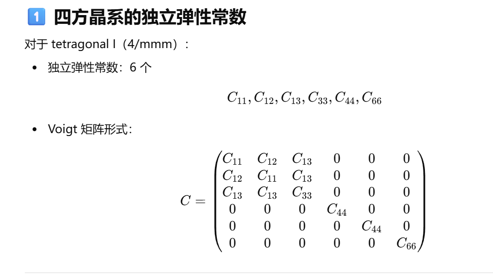
根据线弹性假设,
$$\sigma = C * \varepsilon$$,给出应变,通过线性组合,可以表示出应力,即公式
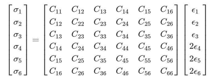
但是,要想使用numpy.linalg.lstsq进行拟合,还需要重新表达一下这关系。
因为lstsq的工作原理是B = A * X,根据已知应变A、应力B,用最小二乘法拟合一个为列向量的系数,X,(这里即Cij)
现在,我们专注于A矩阵的写法。
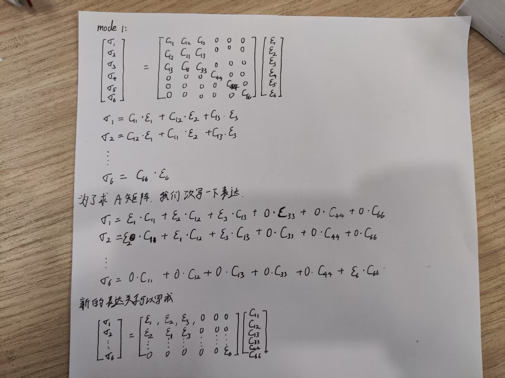
可以看到,应变A矩阵是由所施加的应变,也即是变形模式,以及弹性系数矩阵的形状共同决定的。(Cij矩阵决定了A矩阵的形状,而变形模式决定了它具体的元素值)
有几点需要澄清,待求解的Cij可能不止6个。比如说,7个的时候,需要X列向量是7行,A矩阵是七列吗?显然,不需要也不能。因为一种应变模式只能提供六个线性方程组,6个应力最多只能包含6个弹性系数的有效信息。这也是为什么,低对称晶系需要更多变形模式的原因。因此,我们在选择变形模式的时候,要合理。对于大于6个弹性系数的体系,要让弹性系数间尽量解耦——保证一个变形模式内,涉及的弹性系数最多为6个。通过选取多个变形模式,比如说两种,这样有2个A矩阵,12个方程,把两个A矩阵堆叠起来,就能求解7个Cij了
这里我放上一个具体的脚本,提供一些思路
import numpy as np
from ase.io import read,write
#针对四方相计算弹性常数C11,C12,C13,C33,C44,C66
prim = read('ysz_42.xyz')
ups = [-0.03,-0.01,0.01,0.03]
modes = [0,1]
Ms = []
for mode in modes:
    for up in ups:
        if mode == 0:
            strain_voigt = np.array([up,0.,0.,0.,0.,0.])
            strain_matrix = strain_matrix_1 = np.array([[up, 0., 0.],
                                                        [0., 0., 0.],
                                                        [0., 0., 0.]])
            deform_matrix = np.eye(3)+strain_matrix
            atoms = prim.copy()
            cell_new = deform_matrix @ atoms.cell[:]
            atoms.set_cell(cell_new, scale_atoms=True)
            write('deformcell_{}_{}.xyz'.format(mode,up),atoms)
            #有了应变模式和应变幅度,即可确定M矩阵
            M_matrix = np.array([[up,0.,0.,0.,0.,0.],
                                [0.,up,0.,0.,0.,0.],
                                [0.,0.,up,0.,0.,0.],
                                [0.,0.,0.,0.,0.,0.],
                                [0.,0.,0.,0.,0.,0.],
                                [0.,0.,0.,0.,0.,0.]])
            Ms.append(M_matrix)
        if mode == 1:
            strain_voigt = np.array([0.,0.,up,up,0.,up])
            strain_matrix = np.array([[0., up/2, 0.],
                                      [up/2, 0., up/2],
                                      [0., up/2, up]])
            deform_matrix = np.eye(3)+strain_matrix
            atoms = prim.copy()
            cell_new = deform_matrix @ atoms.cell[:]
            atoms.set_cell(cell_new, scale_atoms=True)
            write('deformcell_{}_{}.xyz'.format(mode,up),atoms)
            M_matrix = np.array([[0.,0.,up,0.,0.,0.],
                                [0.,0.,up,0.,0.,0.],
                                [0.,0.,0.,up,0.,0.],
                                [0.,0.,0.,0.,up,0.],
                                [0.,0.,0.,0.,0.,0.],
                                [0.,0.,0.,0.,0.,up]])
            Ms.append(M_matrix)
Ms = np.array(Ms)
Ms_2d = Ms.reshape(-1, 6)  # 自动把 8*6=48 行展开
print(Ms_2d.shape)  # (48, 6)
print(Ms_2d)
#C_fit, residuals, rank, s = np.linalg.lstsq(Ms_2d, sigma_vec, rcond=None)
代码中的M,就是上述的A矩阵。除此之外,代码是先把变形模式1的不同幅值的A矩阵堆叠起来,然后再把变形模式2的不同幅值的A矩阵堆叠起来。
顺序是没有影响的。本质上就是拟合2 * 4 * 6 = 48个应力应变关系涉及的6个Cij。就是把矩阵行交换,是不影响有效信息的。
最后,有了堆叠后的应变A矩阵和应力向量,简单的使用lstsq拟合即可。
此外,也可以观察到,这些A矩阵中的每一行中,只有一个不为零的值,其实是因为我们的四方晶系比较简单,合适的应变模式选取让Cij之间完全解耦。
这种情况下,如果不嫌弃麻烦,也可以从这个48个方程中挑选出对应的,某个Cij与有些应力的关系,单独拟合。
0K下的弹性系数
0K下DFT计算略过,使用MLIP也不需要跑MD,只需要对变形进行评估得出应力即可。
手动法:
calorine
我们用的小胞不再改变体积。我们需要做的就是施加应变,然后计算应力。
这个过程其实是:(1)弛豫(2)输出应力
我们这里用与nep配套的calorine软件包结合ase进行弛豫。
#对结构进行弛豫并计算应力
import numpy as np
from ase.io import read,write
from ase.units import GPa
from calorine.calculators import CPUNEP
from calorine.tools import relax_structure,get_elastic_stiffness_tensor

prim = read('CONTCARYSZ')
calc = CPUNEP('nep.txt')
#ups = [-0.006,-0.004,-0.002,0.002,0.004,0.006]
ups = [-0.006,-0.002,0.002,0.006]
modes = [0,1]
stresses = []
for mode in modes:
    for up in ups:
        if mode == 0:
            strain_matrix = strain_matrix_1 = np.array([[up, 0., 0.],
                                                        [0., 0., 0.],
                                                        [0., 0., 0.]])
            deform_matrix = np.eye(3)+strain_matrix
            #每次拷贝一下原始结构
            atoms = prim.copy()
            #左乘变形矩阵
            cell_new = deform_matrix @ atoms.cell[:]
            #重新定义胞并缩放原子
            atoms.set_cell(cell_new, scale_atoms=True)
            #为变形后的晶胞绑定计算器
            atoms.calc = calc
            #弛豫结构
            relax_structure(atoms,fmax=0.02,steps=300,minimizer='fire',constant_cell=True,constant_volume=True)
            #输出应力
            stress = np.array(atoms.get_stress())/GPa
            stresses.append(stress)

        if mode == 1:
            strain_matrix = np.array([[0., up/2, 0.],
                                      [up/2, 0., up/2],
                                      [0., up/2, up]])
            deform_matrix = np.eye(3)+strain_matrix
            atoms = prim.copy()
            cell_new = deform_matrix @ atoms.cell[:]
            atoms.set_cell(cell_new, scale_atoms=True)
            atoms.calc = calc
            relax_structure(atoms,fmax=0.02,steps=300,minimizer='fire',constant_cell=True,constant_volume=True)
            stress = np.array(atoms.get_stress())/GPa
            stresses.append(stress)

np.savetxt('stresses.txt',stresses)
# prim.calc = calc
# cij = get_elastic_stiffness_tensor(prim, fmax=0.01,epsilon=0.001)
# print(cij)
calorine自带的cij计算器采用的不是应力应变法,没有深究。
这里结构优化的时候,一定要固定体积和晶胞形状,不然等于没有应变。
import numpy as np
from ase.io import read,write
#针对四方相计算弹性常数C11,C12,C13,C33,C44,C66
seed = '1'
#ups = [-0.006,-0.004,-0.002,0.002,0.004,0.006]
ups = [-0.006,-0.002,0.002,0.006]


modes = [0,1]
Ms = []
for mode in modes:
    for up in ups:
        if mode == 0:
            strain_voigt = np.array([up,0.,0.,0.,0.,0.])
            strain_matrix = strain_matrix_1 = np.array([[up, 0., 0.],
                                                        [0., 0., 0.],
                                                        [0., 0., 0.]])
            #有了应变模式和应变幅度,即可确定M矩阵
            M_matrix = np.array([[up,0.,0.,0.,0.,0.],
                                [0.,up,0.,0.,0.,0.],
                                [0.,0.,up,0.,0.,0.],
                                [0.,0.,0.,0.,0.,0.],
                                [0.,0.,0.,0.,0.,0.],
                                [0.,0.,0.,0.,0.,0.]])
            Ms.append(M_matrix)
        if mode == 1:
            strain_voigt = np.array([0.,0.,up,up,0.,up])
            strain_matrix = np.array([[0., up/2, 0.],
                                      [up/2, 0., up/2],
                                      [0., up/2, up]])

            M_matrix = np.array([[0.,0.,up,0.,0.,0.],
                                [0.,0.,up,0.,0.,0.],
                                [0.,0.,0.,up,0.,0.],
                                [0.,0.,0.,0.,up,0.],
                                [0.,0.,0.,0.,0.,0.],
                                [0.,0.,0.,0.,0.,up]])
            Ms.append(M_matrix)
Ms = np.array(Ms)
Ms_2d = Ms.reshape(-1, 6)  # 自动把 8*6=48 行展开
# print(Ms_2d.shape)  # (48, 6)
# print(Ms_2d)
stress = np.loadtxt('stresses.txt')
# print(stress.shape)
stress = stress.reshape(-1,1)
# print(stress)
cij, residuals, rank, s = np.linalg.lstsq(Ms_2d, stress, rcond=None)


c11 = cij[0][0]
c12 = cij[1][0]
c13 = cij[2][0]
c33 = cij[3][0]
c44 = cij[4][0]
c66 = cij[5][0]

M = c11+c12+2*c33-4*c13
C2 = (c11+c12)*c33-2*c13*c13

B_v = (2*(c11+c12)+c33+4*c13)/9.
G_v = (M+3*c11-3*c12+12*c44+6*c66)/30.
B_r = C2/M
G_r = 15./(18*B_v/C2+6/(c11-c12)+6/c44+3/c66)

B_vrh = (B_v+B_r)/2.
G_vrh = (G_v+G_r)/2.
E = 9*B_vrh*G_vrh/(3*B_vrh+G_vrh)
v = (3*B_vrh-2*G_vrh)/(2*(3*B_vrh+G_vrh))

with open('elastic_{}'.format(seed),'w') as f:
    f.write(str(ups)+'\n')
    f.write(f'C11: {c11}\n')
    f.write(f'C12: {c12}\n')
    f.write(f'C13: {c13}\n')
    f.write(f'C33: {c33}\n')
    f.write(f'C44: {c44}\n')
    f.write(f'C66: {c66}\n')
    f.write(f'E: {E}\n')
    f.write(f'residuals: {residuals}\n')
    f.write(f'rank: {rank}\n')
    f.write(f's: {s}\n')
这个代码只适用于四方相-1,别的需要改动M矩阵以及输出cij时的处理。
有限温度下的弹性系数
首先在npt下保温一段时间,确定平均晶格常数。然后施加变形,在nvt下进行保温求出应力的时间平均。
npt保温
potential   ./nep.txt
minimize fire 1.0e-5 300
velocity    10
time_step   0.5

dump_thermo 5000
dump_exyz 2000 1 1
ensemble npt_scr 10 1500 100 0 0 0 300 300 300 1000
run 100000


dump_thermo 100
dump_exyz 200 1 1 1
ensemble npt_scr 1500 1500 100 0 0 0 300 300 300 1000
run 200000
nvt保温
potential   ./nep.txt
minimize fire 1.0e-5 300
velocity    10
time_step   0.5

dump_thermo 5000
dump_exyz 2000 1 1
ensemble nvt_bdp 10 1500 100
run 100000


dump_thermo 100
dump_exyz 200 1 1 1
ensemble nvt_bdp 1500 1500 100
run 200000